Super Smash Bros. Ultimate is the latest installment of Super Smash Bros., a series of competitive multiplayer games by Nintendo. In Super Smash Bros., players pick from a roster of Nintendo characters and duke it out on a 2D platformer-esque stage. In Smash Ultimate, the roster features 87 unique characters, which, in a 2-player game, makes 7569 total match ups. Each character has different fighting stats and abilities, so each match up is unique.
Statement of Purpose
I want to model the outcome of a match given the characters and the skill level of the players. It would be interesting to see how effective certain characters are at different skill levels. I would also like to know if the stages the matches are played on affect the outcome, or make no difference. The goal of this project is more about interpretation than about raw predictive power.
Data
Source
I sourced my data from smashdata.gg through their Github. The file I downloaded was ultimate_player_database.zip.
Missing Data
Fortunately, smashdata.gg provides us with some insight on why data is missing and how it has been handled. They say, “A lot of tournaments also don’t report full data, meaning game counts and character data have been lost.” Character data is our primary focus, but it seems that this is not dependent on the values themselves, just the tournaments they come from. This means we can assume missing data is missing completely at random, meaning it is not dependent on the values themselves nor any other values in the dataset. Therefore, I’ve decided to remove all the rows where the game data is completely absent. If the game data is present but the character data is absent, then I filled in the value for character with -1, indicating this absence.
Data cleaning
The data from smashdata.gg first needs to be cleaned in order to be used for modeling.
We are given a database file which contains information about sets, tournaments, players, and so on. I am only interested in the set data, and specifically, the game data column in sets. We are given the game data as a json string, so I will extract this to a dataframe.
Code
import sqlite3import numpy as npimport pandas as pdimport jsonimport mathimport randomfrom IPython.display import clear_outputcnx = sqlite3.connect('data/ultimate_player_database.db')query ="SELECT game_data FROM sets WHERE game_data != '[]'"df = pd.read_sql_query(query, cnx)data =list()for k inrange(len(df)):if k %50000==0: clear_output()print("{prop}% complete".format(prop = math.floor(100*k/len(df))))str= df.loc[k][0]whileTrue: id1 =str.find("{") id2 =str.find("}")if (id1 !=-1 ) and (id2 !=-1): new_data = json.loads(str[id1:id2+1]) data.append(new_data)else:breakstr=str[id2+1:]game_df = pd.DataFrame(data).fillna(-1)game_df.to_csv("data/game_data.csv",index =False)clear_output()print("100 % complete")
Now I’ll modify the character data so it is easier to read.
We need to transform our data to be impartial to the winner or loser. We now have winner_id, loser_id, winner_char,loser_char, … ect but what we want is p_1_id,p2_id, p1_char,p2_char, p1_won. Otherwise, we wouldn’t be predicting anything because we would know who won beforehand. Let’s transform our data to add our desired columns.
I want to add a column that gives information about how many games a player has played and won so we can have a sort of “skill” metric. However, we need to be careful about when we transform our data. If we do it across the entire dataset then, for example, the model could deduce that someone with 0 games won has a 0% chance of winning and get 100% accuracy for those values. Someone with 0 games previously won might have a low chance of winning, but it is certainly not zero. So, I’m going to split the ENTIRE dataset in half, then calculate player ratio and skill from that. Then the games played and games won metrics would be independent of both the training and test, and any data points lost in our training / test sets would be missing by random chance.
Code
def transform_games_played(dataframe): p1s =dict(dataframe["p1_id"].value_counts()) p1wins =dict(dataframe[dataframe["p1_won"] ==True]["p1_id"].value_counts()) p2s =dict(dataframe["p2_id"].value_counts()) p2wins =dict(dataframe[dataframe["p1_won"] ==False]["p2_id"].value_counts()) players =set(p1s.keys()).union(set(p2s.keys())) games_played =list()for item in players: totalsum =0 winsum =0if item in p1s.keys(): totalsum += p1s[item]if item in p2s.keys(): totalsum += p2s[item]if item in p1wins.keys(): winsum += p1wins[item]if item in p2wins.keys(): winsum += p2wins[item] games_played.append({"player_id" : item, "games_played" : totalsum, "games_won" : winsum}) games_played_df = pd.DataFrame(games_played)return games_played_dfdef clean_games(given_df,skill_df): games_played_df = transform_games_played(skill_df) output_df = pd.merge(given_df,games_played_df, left_on ="p1_id", right_on ="player_id", how ="left") output_df.rename(columns = {"games_played" : "p1_games_played", "games_won" : "p1_games_won"}, inplace=True) output_df = pd.merge(output_df,games_played_df, left_on ="p2_id", right_on ="player_id", how ="left") output_df.rename(columns = {"games_played" : "p2_games_played", "games_won" : "p2_games_won"}, inplace=True) output_df["p1_games_won"].fillna(0,inplace=True) output_df["p1_games_played"].fillna(0,inplace=True) output_df["p2_games_won"].fillna(0,inplace=True) output_df["p2_games_played"].fillna(0,inplace=True) output_df.reset_index(inplace=True) output_df.drop(columns=["index","player_id_x","player_id_y"],inplace=True)return output_df_skill_df = imp_game_df.sample(frac =0.5, random_state=2049)remaining_df = imp_game_df.drop(_skill_df.index)clean_game_df = clean_games(remaining_df,_skill_df) # The output rows are independent of the games played and won.skill_clean_game_df = clean_games(_skill_df,_skill_df) # The output rows are NOT independent of the games played and won.clean_game_df.to_csv("data/clean_game_data.csv",index=False) # To be used for training/test.skill_clean_game_df.to_csv("data/dependent_skill_data.csv",index =False) # To be used in case we want to create more metrics.
We can now better use our data for fitting models.
Codebook
This codebook identifies each of the variables in cleaned_game_data.csv.
Variable
Description
p1_id
A string identifying the first player.
p2_id
A string identifying the second player.
p1_games_played
An integer indicating how many games the first player has played in dependent_skill_data.csv.
p2_games_played
An integer indicating how many games the second player has played in dependent_skill_data.csv.
p1_games_won
An integer indicating how many games the first player has won in dependent_skill_data.csv.
p1_games_won
An integer indicating how many games the second player has won in dependent_skill_data.csv.
p1_char
A string indicating the character of the first player.
p2_char
A string indicating the character of the second player.
stage
A string identifying the stage the match was played on.
p1_won
A boolean indicating if the first player won.
Exploratory Data Analysis
First, let’s load our data in.
Code
import pandas as pdimport numpy as npimport matplotlib.pyplot as pltimport randomgame_df = pd.read_csv("../Data/data/clean_game_data.csv")skill_data = pd.read_csv("../Data/data/dependent_skill_data.csv")
Correlation Matrix
Let’s start by plotting a correlation matrix between our numeric variables.
We see that p1_games_played and p2_games_played are correlated, meaning players with more games played are more likely to play against each other. We also see that p1_games_played and p1_won are correlated, so games_played might be a good indicator of skill. Let’s explore this further.
“Games Played” as Skill
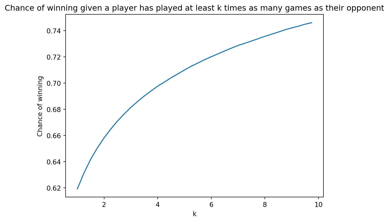
I want to establish that games played may be a good indicator of skill. To do this, I’ll ask the question: How likely are you to beat someone who has played at least k times as many games as you?
Let’s write some code to figure this out.
Code
def k_times_more_games_win_rate(k, df = game_df):return( (len(df[(df["p1_won"] ==True) & (df["p1_games_played"] > k*df["p2_games_played"])]) +len(df[(df["p1_won"] ==False) & (df["p2_games_played"] > k*df["p1_games_played"])]) ) / (len(df[(df["p1_games_played"] > k*df["p2_games_played"])]) +len(df[(df["p2_games_played"] > k*df["p1_games_played"])]) ) )graph = [k_times_more_games_win_rate(n/4) for n inrange(4,40)]plt.plot([(n/4) for n inrange(4,40)],graph)plt.xlabel("k")plt.ylabel("Chance of winning") plt.title("Chance of winning given a player has played at least k times as many games as their opponent") plt.show()print(k_times_more_games_win_rate(1))
0.6192630428086423
This graph justifies the belief that games played is a metric of skill level, because someone with more games played has a higher chance of winning.
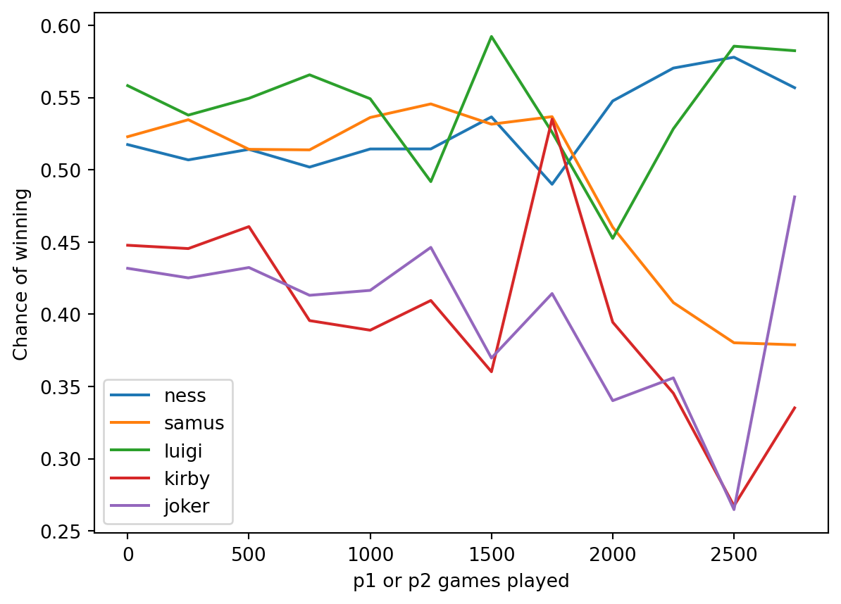
Win Percent vs Skill by Character
I suspect that character win rate might change depending on how skilled a player is. For example, maybe kirby is a really good character until you get to a certain level, at which point they are less viable.
Let’s define some functions that will help us graph win chance against games played.
We see that the variance of these lines increases with games played, likely because there are less players with many games played. We can decipher some trends in these lines visually, like how the mean of Ness and Luigi’s win rate stays relatively constant, though the mean of Joker and Samus’s seem to decrease. This supports our hypothesis that win percent is not constant with respect to skill.
Distribution of Games Played
Let’s verify that there are less players with many games played.
Code
df1 = skill_data[["p1_id","p1_games_played"]].rename(columns = {"p1_id" : "player_id","p1_games_played" : "player_games_played"})df2 = skill_data[["p2_id","p2_games_played"]].rename(columns = {"p2_id" : "player_id","p2_games_played" : "player_games_played"})player_games_played_df = df1.append(df2,ignore_index =True).astype({"player_id" : "string", "player_games_played" : "int32"}).drop_duplicates(ignore_index=True).sort_values("player_games_played").reset_index(drop=True)plt.hist(player_games_played_df["player_games_played"].to_list(),bins=range(0,200,5))plt.title("Histogram of games played")plt.ylabel("count")plt.xlabel("games played")plt.show()#plt.hist(player_games_played_df[player_games_played_df["player_games_played"] >= 200]["player_games_played"].to_list(),bins=range(200,2000,50))#plt.show() - has same 1/x graph
We can see that there are far less players with many games played than with few games played.
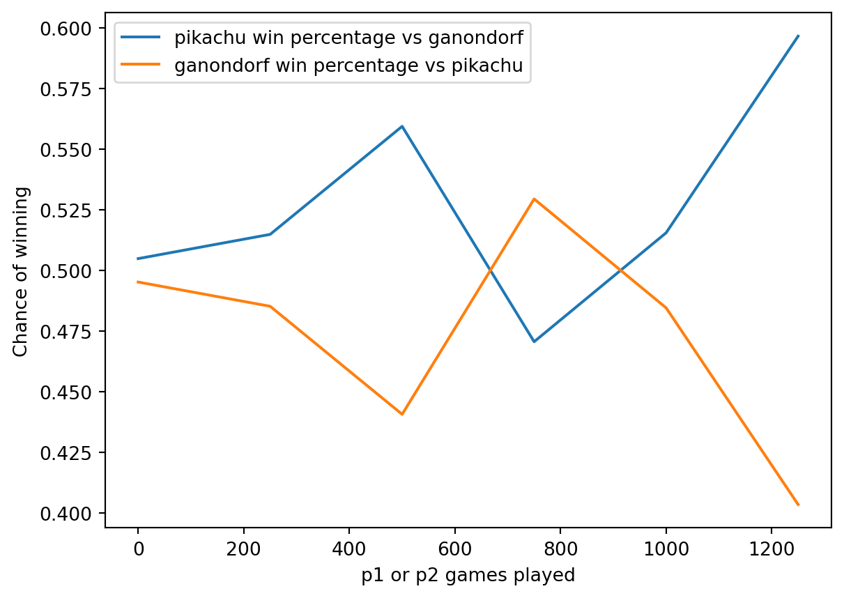
Win Percent vs Skill of Specific Matchups
Finally, I want to look at how the win percents of a matchup of two characters changes with respect to games played.
I’ll modify our previous functions and plot a graph of the win ratios of pikachu versus ganondorf.
Again, we see that the win percentage changes as a function of the skill level of the players.
Overview
We’ve now gathered sufficient information about the relationships between our variables, and have a better idea about which models we can use for fitting our data. It seems as though games played and games won will likely fit a logistic regression, but other variables such as the character data might be need more flexible models.
Fitting Models
Metrics
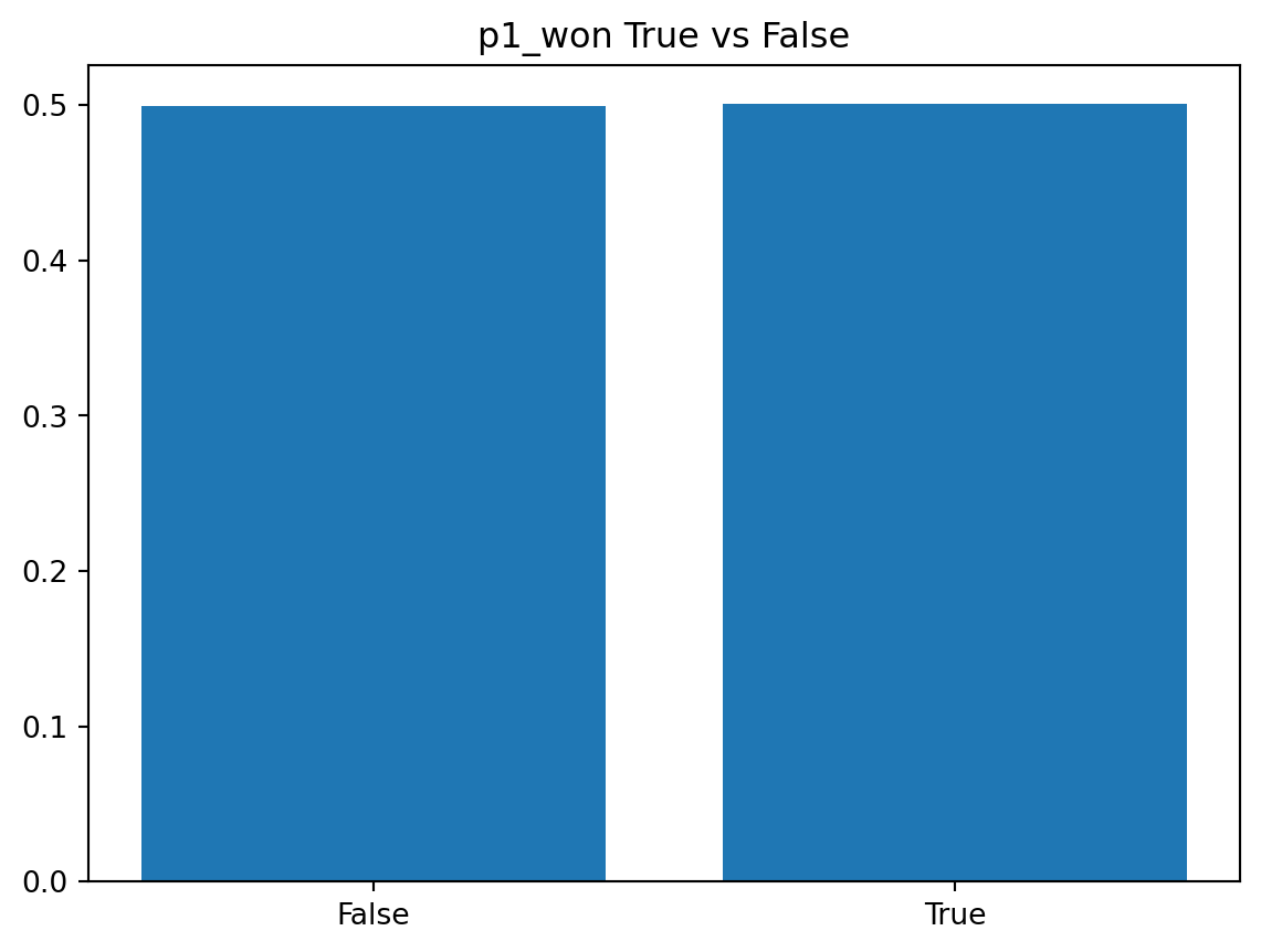
For classification problems, the two metrics to focus on are accuracy and the area under the ROC curve. In general it is better to use roc_auc because it accounts for class imbalances, however it is more difficult to visualize than accuracy. Because I randomized p1_won when I transformed the data, there is no class imbalance present. Because of this, for hyperparameter tuning I’m going to score by accuracy as accuracy is much easier to interpret. Let’s verify that there is no class imbalance:
I dummy-coded some of the categorical variables right away so the data is easier to use.
We need to split our data into a testing set and a training set so we can train our models and evaluate their accuracy. I am going to use a 4:1 ratio, and stratify across our response variable p1_won, so we don’t develop any unexpected imbalances across our training and testing environments.
Code
game_train, game_test = train_test_split(game_data, train_size =0.8, stratify = game_data[["p1_won"]], random_state=2049)# We stratified on our response, p1_won. # This shouldn't make too much of a difference because we randomized which is p1 and p2, however it is still good practice.X = game_train.loc[:,game_train.columns !="p1_won"]y = game_train["p1_won"]game_folded = StratifiedKFold(n_splits=5).split(X,y)
Hyperparameter Tuning
The following block of code will make it easier to save and load models.
Code
def fitmodel(model, filename, df = game_train):ifnot os.path.isfile(filename): model.fit(X,y) joblib.dump(model, filename)else: modeltemp = joblib.load(filename)if (type(model) !=type(modeltemp)) or\ (tuple([k[0] for k in model.steps]) !=tuple([k[0] for k in modeltemp.steps])):print ("\033[93m Warning: model mismatch. Delete the file {filename} and rerun or risk faulty models.\n\033[0m".format(filename=filename)) model = modeltempreturn model
To tune hyperparameters, we need to create a grid of possible values for our models, and select the best set of hyperparameters for each model. To select the best set of hyperparameters, we use cross validation. This process involves “folding” our dataset into many disjoint sets, training a model on these sets, and evaluating each model by using another fold as a testing set. Then, we average these results to get a cross-validated score for each set of hyperparameters. Finding the best cross-validated score should tell us which set of hyperparameters is best for our model.
Elastic Net
In sklearn, there aren’t recipes. Instead, there are pipelines, which works a bit like a recipe and a workflow combined. We can apply transformations to our data including selecting predictors, normalizing variables, and adding models.
To find the best hyperparameters for our models, our first step is to set up a pipeline. Let’s begin by setting up a pipeline for an elastic net.
An elastic net is similar to a linear regression, except it can perform better when overfitting may be present. It combines the strengths of a lasso and ridge regression. For our model, we used a logistic elastic net because it is a classification problem.
I’ve only selected games played and games won for this model, because for the other predictors such as character to be useful, we would need to add interaction terms. To add interaction terms, we would use sklearn.preprocessing.PolynomialFeatures as a step in our pipeline. However, because there are so many characters, my computer runs out of memory when adding these terms. Regardless, an elastic net is probably not the best way to deal with these interactions anyway - a more flexible model like a decision tree or random forest can automatically find interactions between variables. Let’s wait to use a different model before adding these predictors.
Our next step is to create a grid of hyperparameters we want to check. For an elastic net, I’ve chosen to tune l1_ratio and C. C controls the penalty strength of the elastic net, and l1_ratio controls the ratio of l1 to l2 in the elastic net, in other words, how similar the elastic net is to a lasso regression versus a ridge regression. l1_ratio thus takes values between 0.0 and 1.0, while C can take on any non-negative value.
Lastly, we try each combination of variables and pick the model with the best cross validation score. We are going to fold our data with k = 5, and take the average cross-validated score for each combination of hyperparameters. We will then select the highest average score across all hyperparameter combinations.
Code
game_folded = StratifiedKFold(n_splits=5).split(X,y)en_grid_search = GridSearchCV(estimator = en_pipe, param_grid = en_grid, n_jobs =1, cv = game_folded, scoring ='accuracy', error_score =0, verbose =4)en_grid_result = en_grid_search.fit(X[en_predictors],y) # We pass in X[en_predictors] because the result is the same but slightly faster.
Running this code, we find that the best combination of hyperparameters across our search is with l1 = 1.0 and C = 0.01. This has a cross-validated accuracy of 0.643, which is a good start.
A decision tree classifier operates a bit like a game of 20 questions: at each node, the model asks a true-false question, and goes down a branch of the tree. After it has asked enough questions, it assigns a class to an observation.
We perform a similar process as in the elastic net for each of our models. This time, we’re also going to use character and stage data as predictors, and for hyperparameters, we are going to tune max_depth and min_samples_leaf. Both max_depth and min_samples_leaf help with overfitting, which is a big problem in decision trees. max_depth controls the maximum depth of the decision tree, and min_samples_leaf controls the minimum number of samples required to be at a leaf node.
We find that the best max_depth is 10, and the best min_samples_leaf is also 10. Our cross-validated accuracy is 0.647, so this model performs similar to our elastic net. Let’s fit our model and continue.
A random forest classifier works by creating many decision trees and combining their predictions. Each tree in the random forest uses a random set of avalible predictors. Usually, this set has the square root of the total number of predictors. A random forest can perform better than a single decision tree in many cases because it doesn’t tend to overfit the training data.
Again, we repeat our process of creating a pipe, searching through hyperparameters, and fitting a model. Because random forest models many decision trees at once, some of the hyperparameters are the same. For a random forest, I am going to tune the hyperparameters n_estimators and min_samples_leaf, because I found that min_samples_leaf made the biggest difference in the decision tree, and n_estimators, the number of trees in the random forest, can make a big difference on the performance.
Despite 400 trees having the highest mean test score, it is only by .00035, and is computationally twice as expensive as 200 trees, which itself is only higher than 100 trees by .0007. We can always use a higher number of trees to get a marginally better test score, so with discretion, I am going to use 200 trees with min_samples_leaf = 3.
So we get a cross-validation score of 0.673 for our random forest with 200 trees and min_samples_leaf = 3. This is around 3 percent better than our previous models!
Our last model I want to fit is a boosted tree. A boosted tree works similar to a single decision tree, except its branches are weighted and updated iteratively. The model calculates the gradient at each step and updates the tree in the best way possible.
For this model, I would like to tune max_depth and min_samples_leaf, as well as learning_rate and n_estimators. These are a lot of hyperparameters, and a boosted tree is one of the longest models to fit. As we have it now, if I had 4 levels for each of these parameters, GridSearchCV.fit would take around 174 hours to run, which is over a week.
To get around this, I am going to reduce the size of the dataset I am tuning over. This isn’t ideal, because all of these parameters could depend on the size of the dataset, but in our case, we don’t have many options.
Before fitting our chosen model, I’ll also cross-validate it separately with the full dataset, as the cross-validation from the hyperparameter tuning won’t reflect the results of our true chosen model.
We find that the best set of hyperparameters is n_estimators = 500, learning_rate = 0.2, min_samples_leaf = 3, max_depth = 2, with an accuracy of 0.66928.
To find the true cross-validated accuracy of this model, we can cross-valdate with the entire dataset.
Code
gbc_pipe.set_params(boosted_tree__max_depth =2, boosted_tree__n_estimators =500, boosted_tree__learning_rate =0.2, boosted_tree__min_samples_leaf =3)game_folded = StratifiedKFold(n_splits=5).split(X,y)cross_val_score(estimator = gbc_pipe, n_jobs =1, cv = game_folded, X = X, y = y, scoring ='accuracy', error_score =0, verbose =10)
And we find that the model has a cross-validation accuracy of 0.680, our best accuracy yet.
Evaluation
Let’s set up and load our best models in. I want to look at the random forest classifier and the elastic net. The random forest classifier did almost as good as the boosted tree in cross-validation (0.007 difference), and contains information about variable importance, which I want to analyze and interpret. The elastic net provides a good baseline for what we should expect from our model, and lets us more deeply analyze how our numerical predictors effect outcome.
Code
game_train, game_test = train_test_split(game_data, train_size =0.8, stratify = game_data[["p1_won"]], random_state=2049)X = game_train.loc[:,game_train.columns !="p1_won"]y = game_train["p1_won"]X_test = game_test.loc[:,game_train.columns !="p1_won"]y_test = game_test["p1_won"]# We use the same seed so that we get the same testing data as in our model_fitting file. This is important for evaluation.en = joblib.load("../Prediction/models/elastic_net.joblib")rfc = joblib.load("../Prediction/models/random_forest.joblib")rfc.set_params(random_forest__verbose =0)
Metrics
Let’s display our test roc_auc and accuracy.
Code
def get_metrics(model): prediction = model.predict(X_test) actual = y_testprint("Metrics for {model}\n".format(model=model[-1]))print("Accuracy: %0.4f"% accuracy_score(prediction,actual))print("ROC_AUC: %0.4f"% roc_auc_score(prediction,actual))print("\n")get_metrics(en)get_metrics(rfc)
Metrics for LogisticRegression(C=0.01, l1_ratio=1.0, penalty='elasticnet', solver='saga')

Accuracy: 0.6432
ROC_AUC: 0.6432
Metrics for RandomForestClassifier(min_samples_leaf=3, n_estimators=200, n_jobs=4,
                       random_state=420)

Accuracy: 0.6782
ROC_AUC: 0.6782
Model
Accuracy
ROC AUC
Logistic Regression
0.6432
0.6432
Random Forest
0.6782
0.6782
Interestingly, the roc_auc and accuracy is the same for both our models. This is likely because there is no class imabalance present, which further justifies our decision to use accuracy as a scoring metric in our hyperparameter tuning.
The elastic net got an accuracy of 0.6434, and the random forest got an accuracy of 0.6782. We might intepret the difference in these accuracies as the amount that adding the character and stage data affected the score. More precisely, this difference would be the percent of variability in the response explained by the random forest that could not be explained by the elastic net.
Variable Importance
I want to find the variable importance of the predictors in my random forest so I can make some statements about how certain varaibles affect outcome.
Here is a table of the most important variables in the RFC:
To no suprise, the most important predictors are games played and games won for both players. However what is interesting is that the next 8 most important predictors are stage, and only then do we see character data.
The following is speculation from my personal experience. I suspect that stage is an important predictor not because of the stage itself, but because of the kinds of tournaments associated with these stages. I would guess that Pokemon Stadium 2, Town & City, Final Destination, Battlefield, ect. all come up as the most important stages associated with predictive power because these stages are often used in high-level tournaments. If you watch competitive smash, these are the kinds of stages you see top players playing on. This is likely just by preference and standarization in the Smash community, however we see that this preference shows up in our model, which is an interesting result.
Now, I want to look at how character data affects the outcome.
In most cases, we see that if p1_char and p2_char are the same character, they have a similar importance. This is a good thing because we would expect our model to be symmetric, in that, the outcome shouldn’t matter based on who is the first player or the second player.
Because this table only shows how important the variables are and not their relationship to the outcome, it is not possible to tell whether showing up at the top means a character is favorable or unfavorable. However, it is interesting to see which characters yeild the most predictive power.
If we want to interpret this, we might say that characters towards the top are the least balanced (for their benefit or detriment), and characters towards the bottom are the most balanced. Let’s see which characters have the least predictive power.
We see names like Bowser, Ness, Palutena, Wolf, Yoshi, and more come up first.
Characters near the bottom of the list include Olimar, Pit, Simon, and Daisy. We might interpret these as some of the most balanced characters.
Character Matchups
Now that our model is fit, we can try comparing some characters. When my friend and I first started playing Smash, I would often play Ness and he would usually play Kirby. Let’s try to predict who has the edge in this matchup.
Neither of us have competed in any tournaments, so I’m going to keep our games played and games won at zero.
We now get False. This is what we would expect, because our model should be symmetric around p1 and p2. Looks like I had an advantage!
Recently, we’ve switched up our characters, and he has been beating my Villager as Ganondorf. Let’s see if Ganondorf has an edge against Villager, or if I just need to work on my skills.
False means that the second player won, so Ganondorf is favorable in this matchup. Let’s swap the characters to make sure the model symmetric around p1 and p2.
And as expected, the model is symmetric. Looks like my friend had the edge after all!
Conclusion
I would say that we adequately answered many of our initial questions. We found that stage data is (surprisingly!) an important predictor, and that certain characters are more balanced than others. Furthermore, even though the goal of this project isn’t prediction, our accuracy of 67.8% for our random forest model was fairly good considering the variance in games of this type. If the outcome of a match was near certain, then Smash Ultimate probably wouldn’t be a very fun game anyways. I’m sure we could improve this accuracy further, however, there may simply not be many more trends in the data that we could exploit for our models.
I wanted this project to analyze the skill level of players with respect to their characters, which is why I included data about their games played and games won. Realistically though, my models would only work for new predictions within the same dataset, because the number of games played and games won is dependent on the size of the dataset itself. It is possible I could have scaled and normalized these predictors to work with datasets of varying sizes, however I did not think that was nessecary given that the goal of this project is interpretation.
If I were to expand on this project, I would like to add an interactive component that lets you input match statistics and see the predicted winner of the match. I think this would better answer the question of which characters are better at certain skill levels, and help me pick the best characters to use against my friends!


")